Introduction

There are a number of tasks in numerical processing that are routinely handled with Fourier techniques. One of these is filtering for the removal of noise from a “corrupted” signal¹.

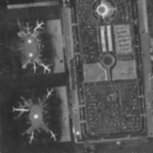
Let’s prepare an image to our experiments. We start with uncorrupted signal $u(t)$. We can take the following image, 512px*512px, as an example:

Pic.1. Original image, $u(t)$

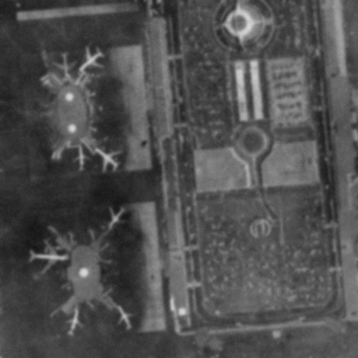
First, the apparatus may not have a perfect “delta-function” response, so that the true signal $u(t)$ is convolved with (smeared out by) some known response function $r(t)$ to give a smeared signal $s(t)$,

\begin{equation} s(t) = \int_{-\infty}^\infty r(t-\tau)u(\tau)d\tau \label{eq:st} \end{equation} or \begin{equation} S(f) = R(f)U(f) \label{eq:Sf} \end{equation} where $S,R,U$ are the Fourier transforms of $s,r,u$ respectively.

Let us use the Gaussian distribution as the response function, and, to be more specific, use 2 dimensions $t_1$ and $t_2$ for $t$: \begin{equation} r(t_1,t_2) = \frac{e^{-(t_1^2 + t_2^2)/a^2}}{a^2\pi}, \quad a=0.2 \label{eq:rt} \end{equation}

Use Imagemagick to perform this task:

convert 5.3.02.png -gaussian-blur 0x2 5.3.02.gaus.png

Note than you may need to rebuild it to use it’s HDRI feature:

sudo apt-get install fftw-dev libjpeg62-dev
sudo apt-get install libfftw3-3 libfftw3-dev
apt-get source imagemagick
cd im*
./configure --enable-hdri --with-jp2=yes --with-jpeg=yes --with-lqr --with-fftw=yes
make install
sudo ldconfig /usr/local/lib

Pic.2. Smeared image, $s(t)$

Second, the measured signal may contain an additional component of noise $n(t)$. So the result, currupted signal $c(t)$, contains the following two components: \begin{equation} c(t) = s(t) + n(t) \label{eq:ct} \end{equation}

Add a Perlin noise by running a Perlin-noise generator:

perlin 512x512 -n poisson -a 2 noise.png

Pic.3. Noise, $n(t)$

To get the result use the Imagemagick’s special composition method:

convert noise.png -normalize  +level 30,70% noise.30-70.png
convert 5.3.02.gaus.png noise.30-70.png -compose Mathematics -define compose:args='0,1,1,-0.5' -composite 5.3.02.corrupt.png

Pic.4. Corrupted image, $c(t) = s(t) + n(t)$

We’ve done with the image preparation. Now let’s get deep into some formulas.

Fourier transform

A physical process can be described either in the time domain, by the values of some quantity $h$ as a function of time $t$, e.g., $h(t)$, or else in the frequency domain, where the process is specified by giving its amplitude $H$ (a complex number indicating phase also), as a function of frequency $f$, that is $H(f)$, with $-\infty < f < \infty$. For many purposes it is useful to think of $h(t)$ and $H(f)$ as being two different representations of the same function. One goes back and forth between these two representations by means of the Fourier transform equations,

$\begin{equation} \begin{aligned} H(f) &= \int_{-\infty}^{\infty}h(t)e^{2\pi ift}dt\\ h(t) &= \int_{-\infty}^{\infty}H(f)e^{-2\pi ift}df \end{aligned} \label{eq:f} \end{equation}$

We estimate the Fourier transform of a function from a finite number of its sampled points. Suppose that we have $N$ consecutive sampled values \begin{equation} h_k \equiv h(t_k), \qquad t_k \equiv k\Delta, \qquad k = 0, 1, 2, \ldots, N − 1 \label{eq:h_k} \end{equation} Here $k$ represents coordinates $(k_1,k_2)$ on the image, $k_1 \in [0..511]$, $k_2 \in [0..511]$, and $h_k$ – image brightness at these points. $\Delta$ is a “one pixel” interval.

As you see we are not dealing with the exactly time domain, instead we treat image as a signal, parameterized with 2-dimentional parameter $t = (t_1,t_2)$.

In this case the representation of this signal in frequency domain, discrete Fourier transform of the $N$ points $h_k$, will be \begin{equation} H_n \equiv \sum_{k=0}^{N-1}h_ke^{2\pi ikn/N} \label{eq:four_H_n} \end{equation}

The formula for the discrete inverse Fourier transform, which recovers the set of $h_k$’s from the $H_n$’s is: \begin{equation} h_k = \frac{1}{N} \sum_{k=0}^{N-1}H_ne^{-2\pi ikn/N} \label{eq:four_h_k} \end{equation}

Now get back to our problem.

Optimal filter

To deconvolve the effects of the response function $r$ \eqref{eq:rt} and when noise \eqref{eq:ct} is present, we have to find the optimal filter, $\phi(t)$ or $\Phi(f)$, which, when applied to the measured signal $c(t)$ or $C(f)$, and then deconvolved by $r(t)$ or $R(f)$, produces a signal $\widetilde{u}(t)$ or $\widetilde{U}(f)$ that is as close as possible to the uncorrupted signal $u(t)$ or $U(f)$, see \eqref{eq:Sf}. In other words we will estimate the true signal $U$ by \begin{equation} \widetilde{U}(f) = \frac{C(f)\Phi(f)}{R(f)} \label{eq:Uf} \end{equation}

To get the closest $\widetilde{U}$ to $U$, we ask in this example that they would be close in the least-square sense \begin{equation} \int_{-\infty}^{\infty}|\widetilde{u}(f)-u(f)|^2dt = \int_{-\infty}^{\infty}|\widetilde{U}(f)-U(f)|^2df \quad \text{is minimized.} \label{eq:Ufmin} \end{equation}

Substituting equations \eqref{eq:Uf} and \eqref{eq:ct}, the right-hand side of \eqref{eq:Ufmin} becomes

$\begin{equation} \begin{aligned} &\int_{-\infty}^{\infty}\left|\frac{[S(f)+N(f)]\Phi(f)}{R(f)} - \frac{S(f)}{R(f)}\right|^2df\\ = &\int_{-\infty}^{\infty}|R(f)|^{-2}\left\{|S(f)|^2|1-\Phi(f)|^2 + |N(f)|^2|\Phi(f)|^2 \right\}df \end{aligned} \label{eq:eq1} \end{equation}$

The signal $S$ and the noise $N$ are uncorrelated, so their cross product, when integrated over frequency f, gave zero. This is practically the definition of what we mean by noise.

The expression \eqref{eq:eq1} will be a minimum if and only if the integrand is minimized with respect to $\Phi(f)$ at every value of $f$. Let us search for such a solution where $\Phi(f)$ is a real function. Differentiating with respect to $\Phi$, and setting the result equal to zero gives \begin{equation} \Phi(f) = \frac{|S(f)|^2}{|S(f)|^2 + |N(f)|^2} \label{eq:Phidiff} \end{equation}

This is the formula for the optimal filter $\Phi(f)$.

Notice that equation \eqref{eq:Phidiff} involves $S$, the smeared signal, and $N$, the noise. The two of these add up to be $C$, the measured signal. Equation \eqref{eq:Phidiff} does not contain $U$, the “true” signal. This makes for an important simplification: The optimal filter can be determined independently of the determination of the deconvolution function that relates $S$ and $U$.

To determine the optimal filter from equation \eqref{eq:Phidiff} we need some way of separately estimating $|S|^2$ and $|N|^2$. There is no way to do this from the measured signal $C$ alone without some other information, or some assumption or guess.

We could obtain the extra information in the following way. For example, we can sample a long stretch of data $c(t)$ and plot its one-sided power spectral density (PSD) using equation \begin{equation} P_h(f) \equiv |H(f)|^2 + |H(-f)|^2 = 2|H(f)|^2 \qquad 0 \leq f < \infty, \quad h(t)\in\R \label{eq:PSD} \end{equation}

The relation between the discrete Fourier transform of a set of numbers and their continuous Fourier transform when they are viewed as samples of a continuous function sampled at an interval $\Delta$ can be rewritten as¹

\begin{equation} H(f_n) \approx \Delta H_n \label{eq:approx_delta} \end{equation}

where $f_n$ is given by

\begin{equation} f_n \equiv \frac{n}{N\Delta}, \qquad n=-\frac{N}{2},\ldots,\frac{N}{2} \label{eq:fn} \end{equation}

Some more steps

to be arranged…

FFT transform with imagemagick

convert 5.3.02.corrupt.png -fft  +depth \
          \( -clone 0 -write magnitude.png +delete \) \
          \( -clone 1 -write phase.png +delete \) \
          null:
convert 5.3.02.corrupt.png -fft  +depth \
          \( -clone 0 -auto-level -evaluate log 10000 -write magnitude_log.png +delete \) \
          \( -clone 1 -write phase.png +delete \) \
          null:

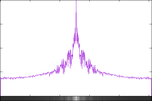
im_profile magnitude_log.png magnitude_log_profile.png
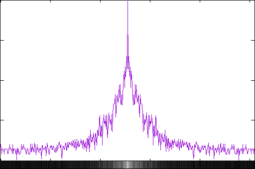
im_profile -v magnitude_log.png magnitude_log_profile_v.png

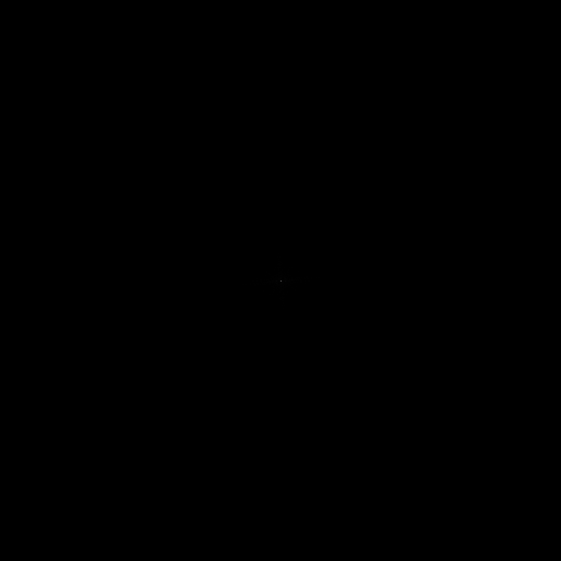
Pic.5. FFT magnitude, mostly black with a single white dot in the middle

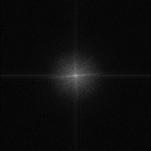
Pic.6. FFT magnitude log scale

Pic.7. Log magnitude profile

Pic.8. Log magnitude vertical profile

Pic.9. FFT phase

Bibliography

Press, William H., Teukolsky, Saul A., Vetterling, William T. & Flannery, Brian P. (1992). Numerical Recipes in C (2Nd Ed.): The Art of Scientific Computing. Cambridge University Press ↩ ↩²